Convolutional Neural Network (CNN)

In this blog, I will discuss Convolutional Neural Networks (CNNs) and demonstrate how to build a neural network for digit image classification.

Brief overview of CNN and its applications

Convolutional Neural Networks (CNNs) are deep learning models designed for image processing. They are used in image classification, object detection, image segmentation, facial recognition, autonomous vehicles, and enhancing text data processing in natural language processing.

Loading and Preprocessing the MNIST Dataset

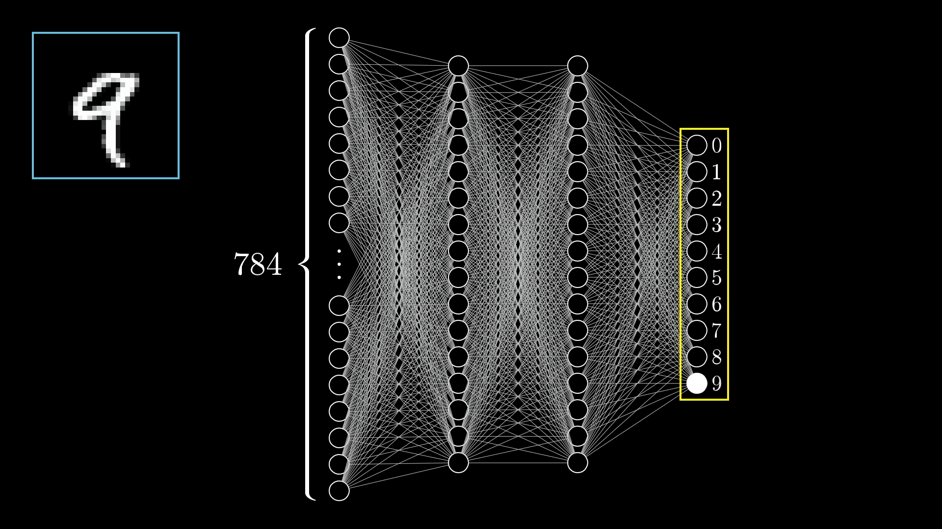
To start building our CNN model, the first step is to load and preprocess the MNIST dataset. The MNIST dataset consists of 60,000 training images and 10,000 testing images of handwritten digits, each of size 28x28 pixels.

Loading the Dataset:

We use the mnist module from tensorflow.keras.datasets to load the dataset. The load_data() function returns four NumPy arrays: the training images (trainX), training labels (trainY), testing images (testX), and testing labels (testY).

from tensorflow.keras.datasets import mnist

# load train and test dataset
(trainX, trainY), (testX, testY) = mnist.load_data()

Reshaping and Encoding the Data:

Since CNNs expect the input data to have a single color channel, we need to reshape the data. The reshape() function modifies the shape of the images to (28, 28, 1).

Additionally, the labels need to be one-hot encoded, converting the integer labels into binary class matrices using the to_categorical() function from tensorflow.keras.utils.

from tensorflow.keras.utils import to_categorical

# reshape dataset to have a single channel
trainX = trainX.reshape((trainX.shape[0], 28, 28, 1))
testX = testX.reshape((testX.shape[0], 28, 28, 1))

# one hot encode target values
trainY = to_categorical(trainY)
testY = to_categorical(testY)

Preparing Pixel Data

Before feeding the MNIST dataset into our Convolutional Neural Network (CNN), it's crucial to preprocess the pixel values to ensure the model performs optimally. This step involves normalizing the pixel values to a range that the neural network can handle more efficiently.

Converting Pixel Values to Floats:

The pixel values in the MNIST dataset are originally integers ranging from 0 to 255. To normalize these values, we first need to convert them to floats. This conversion ensures that subsequent operations, like division for normalization, are performed correctly.

# convert from integers to floats
train_norm = train.astype('float32')
test_norm = test.astype('float32')

Normalizing to Range 0-1:

Neural networks perform better when input values are normalized. In this case, we scale the pixel values from the original range of 0-255 to a range of 0-1. This is done by dividing each pixel value by 255.0.

# normalize to range 0-1
train_norm = train_norm / 255.0
test_norm = test_norm / 255.0
# return normalized images
return train_norm, test_norm

Complete Function:

# scale pixels
def prep_pixels(train, test):
    # convert from integers to floats
    train_norm = train.astype('float32')
    test_norm = test.astype('float32')
    # normalize to range 0-1
    train_norm = train_norm / 255.0
    test_norm = test_norm / 255.0
    # return normalized images
    return train_norm, test_norm

Defining the CNN Model

1.Convolutional Layer:

• The first layer is a 2D convolutional layer with 32 filters, a kernel size of 3x3, and ReLU activation function. This layer uses the 'he_uniform' initializer for the kernel weights and expects input images of shape (28, 28, 1).

model.add(Conv2D(32, (3, 3), activation='relu', kernel_initializer='he_uniform', input_shape=(28, 28, 1)))

2.Max Pooling Layer:

• Following the convolutional layer, we add a max pooling layer with a pool size of 2x2. This layer reduces the spatial dimensions of the feature maps, which helps to decrease computational load and control overfitting.

model.add(MaxPooling2D((2, 2)))

3.Flatten Layer:

• Next, we flatten the 2D feature maps into a 1D vector. This step prepares the data for the fully connected layers.

model.add(Flatten())

4.Fully Connected (Dense) Layer:

• We add a dense layer with 100 units and ReLU activation. This layer further processes the features extracted by the convolutional layers.

model.add(Dense(100, activation='relu', kernel_initializer='he_uniform'))

5.Output Layer:

• The final layer is a dense layer with 10 units and a softmax activation function. This layer outputs the probabilities for each of the 10 digit classes.

model.add(Dense(10, activation='softmax'))

Compiling the Model:

After defining the model architecture, we need to compile the model. Compilation involves specifying the optimizer, loss function, and evaluation metrics. We use the Stochastic Gradient Descent (SGD) optimizer with a learning rate of 0.01 and momentum of 0.9. The loss function is categorical cross-entropy, suitable for multi-class classification tasks. We also specify accuracy as the evaluation metric.

Complete Function:

# define cnn model
def define_model():
    model = Sequential()
    model.add(Conv2D(32, (3, 3), activation='relu', kernel_initializer='he_uniform', input_shape=(28, 28, 1)))
    model.add(MaxPooling2D((2, 2)))
    model.add(Flatten())
    model.add(Dense(100, activation='relu', kernel_initializer='he_uniform'))
    model.add(Dense(10, activation='softmax'))
    # compile model
    opt = SGD(learning_rate=0.01, momentum=0.9)
    model.compile(optimizer=opt, loss='categorical_crossentropy', metrics=['accuracy'])
    return model

Evaluating the Model with K-Fold Cross-Validation

To ensure our Convolutional Neural Network (CNN) model generalizes well to unseen data, we evaluate its performance using K-fold cross-validation. This technique involves splitting the training data into K subsets (folds), training the model on K-1 folds, and validating it on the remaining fold. This process is repeated K times, with each fold used exactly once for validation.

Setting Up K-Fold Cross-Validation:

We use the KFold class from sklearn.model_selection to create the K-fold splits. Here, we specify 5 folds and enable shuffling with a fixed random seed for reproducibility.

from sklearn.model_selection import KFold

# prepare cross validation
kfold = KFold(n_folds, shuffle=True, random_state=1)

Training and Evaluating the Model:

For each fold, we:

1. Define a new instance of the CNN model.
2. Split the data into training and validation sets based on the current fold.
3. Train the model on the training set for 10 epochs with a batch size of 32.
4. Evaluate the model on the validation set and store the accuracy score and training history.

# enumerate splits
for train_ix, test_ix in kfold.split(dataX):
    # define model
    model = define_model()
    # select rows for train and test
    trainX, trainY, testX, testY = dataX[train_ix], dataY[train_ix], dataX[test_ix], dataY[test_ix]
    # fit model
    history = model.fit(trainX, trainY, epochs=10, batch_size=32, validation_data=(testX, testY), verbose=0)
    # evaluate model
    _, acc = model.evaluate(testX, testY, verbose=0)
    print('> %.3f' % (acc * 100.0))
    # stores scores
    scores.append(acc)
    histories.append(history)

Complete Function:

# evaluate a model using k-fold cross-validation
def evaluate_model(dataX, dataY, n_folds=5):
    scores, histories = list(), list()
    # prepare cross validation
    kfold = KFold(n_folds, shuffle=True, random_state=1)
    # enumerate splits
    for train_ix, test_ix in kfold.split(dataX):
        # define model
        model = define_model()
        # select rows for train and test
        trainX, trainY, testX, testY = dataX[train_ix], dataY[train_ix], dataX[test_ix], dataY[test_ix]
        # fit model
        history = model.fit(trainX, trainY, epochs=10, batch_size=32, validation_data=(testX, testY), verbose=0)
        # evaluate model
        _, acc = model.evaluate(testX, testY, verbose=0)
        print('> %.3f' % (acc * 100.0))
        # store scores
        scores.append(acc)
        histories.append(history)
    return scores, histories

Visualizing Learning Curves

To gain insights into how well our Convolutional Neural Network (CNN) model is training and generalizing, we can visualize the learning curves for both loss and accuracy over epochs. These curves help us understand the model's performance on the training and validation sets during the training process.

Plotting Learning Curves:

We use the matplotlib.pyplot library to create plots that display the training and validation loss and accuracy for each epoch. The summarize_diagnostics() function handles this task by iterating over the training histories recorded during cross-validation.

1. Loss Curves:
   • The first subplot displays the cross-entropy loss for both the training and validation datasets.
   • This helps us see how the model's loss decreases over time and whether it converges.
2. Accuracy Curves:
   • The second subplot shows the classification accuracy for both the training and validation datasets.
   • This illustrates how the model's accuracy improves over time.

from matplotlib import pyplot as plt

# plot diagnostic learning curves
def summarize_diagnostics(histories):
    for i in range(len(histories)):
        # plot loss
        plt.subplot(2, 1, 1)
        plt.title('Cross Entropy Loss')
        plt.plot(histories[i].history['loss'], color='blue', label='train')
        plt.plot(histories[i].history['val_loss'], color='orange', label='test')
        plt.legend(['train', 'test'], loc='upper right')

        # plot accuracy
        plt.subplot(2, 1, 2)
        plt.title('Classification Accuracy')
        plt.plot(histories[i].history['accuracy'], color='blue', label='train')
        plt.plot(histories[i].history['val_accuracy'], color='orange', label='test')
        plt.legend(['train', 'test'], loc='upper right')

    plt.show()

Conclusion

In this blog post, we explored the process of building and evaluating a Convolutional Neural Network (CNN) for classifying handwritten digits from the MNIST dataset. We covered the steps of loading and preprocessing the data, defining the CNN model, and evaluating its performance using K-fold cross-validation. Additionally, we visualized learning curves to gain insights into the model's training process.

By following these steps, we demonstrated how CNNs can effectively learn and generalize from image data, achieving high accuracy in digit classification. This foundational knowledge can be applied to various other image classification tasks, showcasing the power and versatility of CNNs in computer vision applications.