Machine Learning Models in Network Security

Introduction

Information system security is increasingly critical as digital transformation expands and cyber-attacks grow in complexity. While greater connectivity and widespread device usage have enabled unprecedented access to information and services, they have also introduced new vulnerabilities. Intrusion Detection Systems (IDS) play a big role in monitoring network traffic and identifying suspicious activity, but traditional IDS struggle to keep pace with modern cyber threats.

Artificial Intelligence (AI) and Machine Learning (ML) offer promising solutions to enhance intrusion detection by improving adaptability and detection accuracy. This study explores the application of ML techniques to IDS using the widely adopted NSL-KDD dataset, a benchmark for evaluating intrusion detection models. By analyzing different ML approaches and their effectiveness in detecting various network attacks, this research aims to contribute to the development of more robust and flexible cybersecurity defenses aligned with current industry trends.

Problem Description

The rising number of cyberattacks shows a significant threat to network security worldwide. Although traditional intrusion detection systems (IDS) have been widely used to identify threats, they often suffer from high false positives, limited adaptability to new attack types, and high maintenance costs. These limitations highlight the need for more flexible and intelligent detection approaches.

Machine learning (ML) offers a promising solution by learning patterns and anomalies from data. However, its effectiveness depends on data quality, feature selection, and robust algorithm choice. Despite being an improvement over KDD’99, the NSL-KDD dataset still faces challenges such as class imbalance, outdated attack samples, and limited representation of emerging threats.

This research applies multiple ML techniques to the NSL-KDD dataset to identify effective models for intrusion detection, with the aim of improving IDS accuracy, efficiency, and adaptability against evolving cyber threats.

Scope

The objective of this project is to examine the use of machine learning techniques for intrusion detection using the NSL-KDD dataset. The study focuses on exploratory data analysis to understand dataset structure and intrusion characteristics, and on evaluating several classification models, including Decision Trees, Random Forests, Support Vector Machines (SVM), and Neural Networks.

Model performance is assessed using accuracy, precision, recall, and F1 score to identify the most effective approaches for detecting different types of intrusions. The research also acknowledges the limitations of the NSL-KDD dataset, particularly its representativeness of real-world traffic and the evolving nature of cyber threats. While deployment in real network environments is outside the project scope, the study aims to provide valuable theoretical insights into the strengths and limitations of machine learning–based intrusion detection systems.

Research Questions

Main Question: How can Artificial Intelligence and Machine Learning be leveraged to improve the detection of network intrusions and enhance cybersecurity defences using the NSL-KDD dataset?

Sub Questions:

• What are the fundamental AI and ML concepts and techniques essential for developing an effective intrusion detection system?
• How does Exploratory Data Analysis (EDA) contribute to understanding the NSL-KDD dataset, and what insights can it provide to inform the development of a moreaccurate intrusion detection model?
• What are some effective machine learning models for intrusion detection incybersecurity, and how do they compare in terms of accuracy, performance, andscalability when applied to the NSL-KDD dataset?

Question 1

What are the fundamental AI and ML concepts and techniques essential for developing an effective intrusion detection system?

Artificial Intelligence (AI): Artificial intelligence (AI) is the capacity of a computer or robot under computer control to carry out operations typically performed by intelligent things. The phrase is commonly used to describe the work of creating artificial intelligence systems that possess like a human ability in areas like reasoning, meaning-finding, generalization, and experience-based learning. (Copeland, 2024)

Machine Learning (ML): Machine learning is a subset of artificial intelligence (AI). It includes image recognition systems, self-driving cars, and products like Amazon’s Alexa. This involves using data and algorithms to emulate the way humans learn enabling machines to do precise predictions, classifications, or the extraction of insights driven by data. Machine learning is about teaching a computer by feeding it lots of data enabling it toguess outcomes, spot patterns, or sort data. There are three kinds of machine learning: supervised, unsupervised, and reinforcement learning. (Staff, 2023)

Supervised learning: Supervised learning is a type of machine learning that is expected to be the most used in businesses, as per Gartner, a business consulting company. This method is being used by providing the models past data. The machine gets both the input and expected output. Then, it processes these to make its future outputs as accurate as possible. Methods like neural networks, decision trees, and linear regression are common in supervised learning. In supervised learning, the machine is guided, or "supervised," during its learning. It's given labelled data as the outcome it needs to learn, and other data as input features to work with. (Staff, 2023)

Unsupervised learning: Unsupervised learning, unlike supervised learning, doesn't rely on labelled training sets. Instead, it allows the machine to discover less apparent patterns in the data by itself. Algorithms commonly used in unsupervised learning include Hidden Markov models, k- means clustering, hierarchical clustering, and Gaussian mixture models. Prediction modelling is one of the many uses for unsupervised learning. It is frequently used for association (finding the rules that connect these groups) and clustering, which groups objects according to their characteristics. Organizing inventory based on manufacturing or sales metrics, classifying customers based on their purchasing patterns, and identifying connections within customer data (such as patterns in the purchases of goods) are a few real-world examples. (Staff, 2023)

Reinforcement learning: One kind of machine learning that closely resembles how people learn is called reinforcement learning. This method involves an algorithm, or "agent," that learns through interactions with its surroundings and the provision of positive or negative rewards. Q-learning, deep adversarial networks, and temporal difference are important algorithms in this field. For example, in a game where we want a car to reach the finish line as soon as possible, we would let the car explore the field by itself and reward it when going the correct direction and take away the rewards when going the wrong direction. This lets the model do the correct job without providing it with any data. (Staff, 2023) Several machine learning models can be especially useful when analyzing Zeek logs for anomaly detection. Zeek logs are a rich source of network data, and the choice of model depends on the specific aspects of network traffic that is being captured. Here are some models that are commonly used:

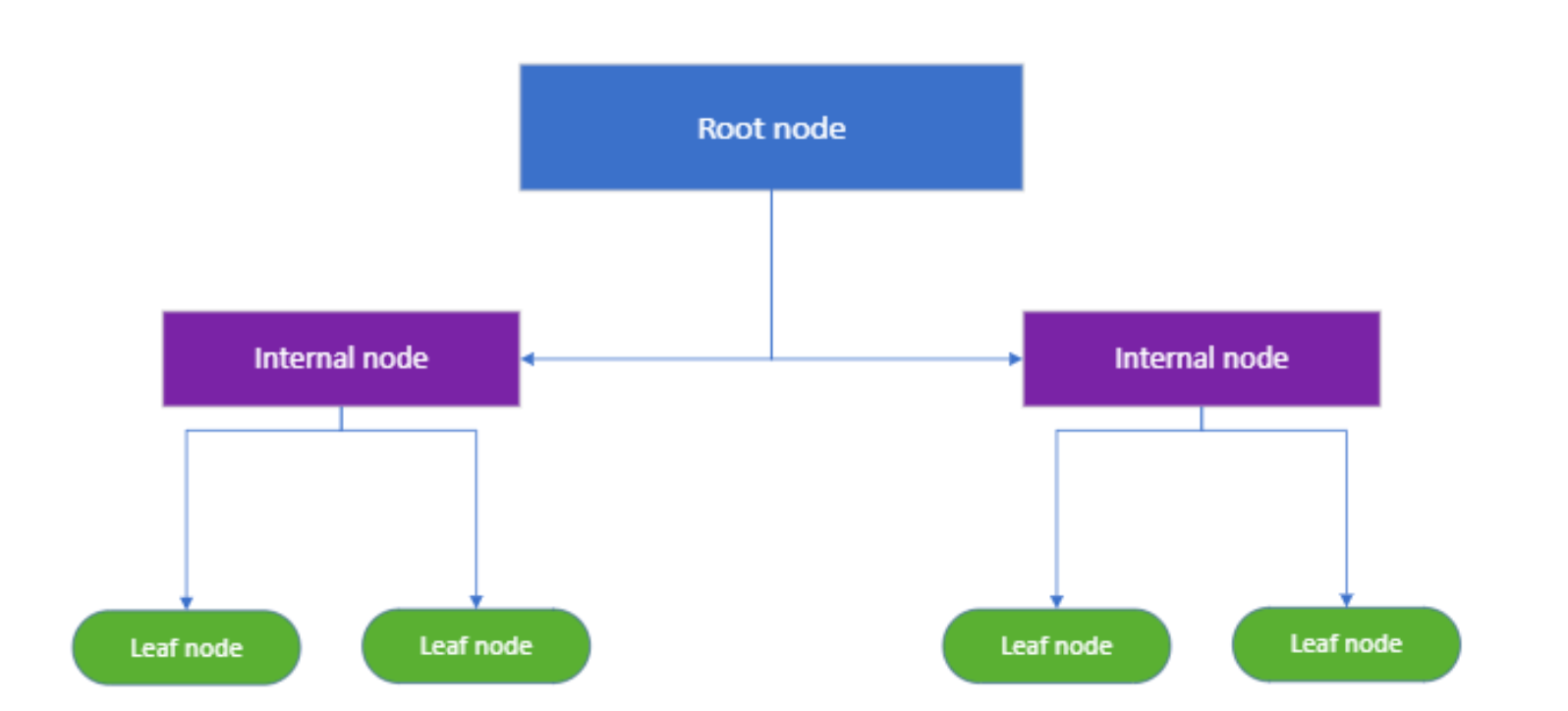
Decision Trees: Decision trees are a type of supervised machine learning algorithm that is used for classification and regression tasks. They make decisions based on asking a series of questions. Structure of a decision trees

• Root Node: This is where the tree starts.
• Splitting: dividing the node into 2 or more sub-nodes based on certain conditions.
• Decision/Internal Node: After the first split, each sub-node becomes a decision/Internal node and can be split further.
• Leaf Node: Last nodes that have no further splits.

The diagram (Figure 1 Structure of a Decision Tree) clearly visualizes each component of a decision tree, showing how data is segmented at different levels based on diverse conditions until a decision is reached at the leaf nodes.

How to choose the best attribute at each node?

There are many techniques for choosing the best attribute at each node in decision tree models. Information gain and Gini impurity are two widely used methods. These techniques assess the effectiveness of each potential next split by categorizing data into classes. To understand how these methods work, it is essential to start with the concept of entropy. Entropy is a measure of the impurity in a set of data. It helps to determine how a decision tree should split the data at each node

Numpy

In order to start working with machine learning models, I need to learn Numpy. Numpy is a library in Python that simplifies working with arrays. Here are some of the things that I learned about Numpy: numpy.where: To find a value inside an array. numpy.ones((x,x)): To generate a matrix (x columns, x rows). numpy.zeros((6,6)): This creates 6*6 matrix all zeros. numpy.max(x): Get the maximum value in an array. x.transpose(): To change from a row vector to a column vector. numpy.sum(x): Get the sum of x (NumPy: The Absolute Basics for Beginners — NumPy v1.26 Manual, 2023)

Tensorflow

TensorFlow is an open-source library for machine learning, flexible tools for building and training models to derive insights and predictions from data. I will go through some of the basics in order to start designing my own models to analyze zeek traffic.

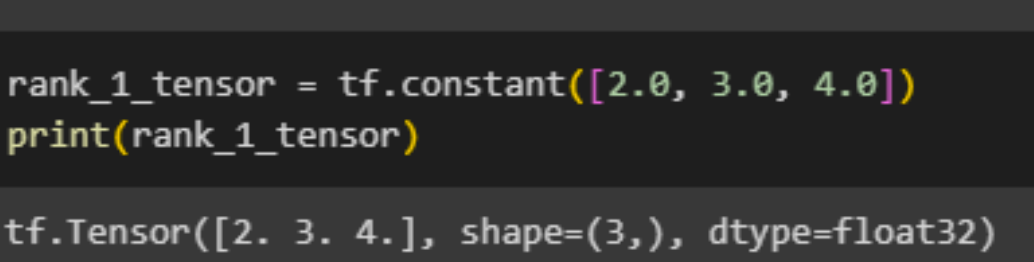
This is how to create a Tensor with multiple float variables: x = tf.Variable(initial_value=[10., 20., 30.], name='float_tensor')

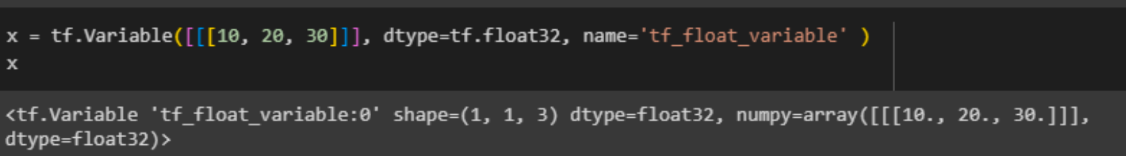
In order to add a new dimension to a Tensor, we can add [] to the values: x = tf.Variable([[10, 20, 30]], dtype=tf.float32 )

Move x to 3 dimensions: x = tf.Variable([[[10, 20, 30]]], dtype=tf.float32, name='tf_float_variable' )

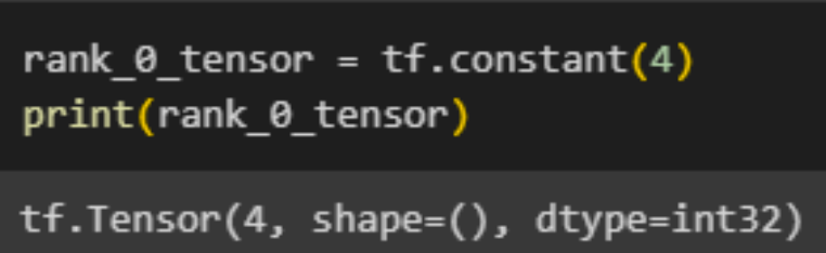
Let’s print the value of x:

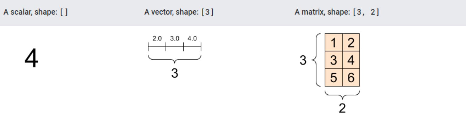
This is a 'scalar' or 'rank-0' tensor. A scalar consists of just one value and does not have any 'axes'.

"A 'vector' or 'rank-1' tensor is similar to a list of values. It has one axis:"

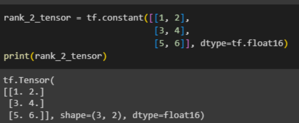
A 'matrix' or 'rank-2' tensor is characterized by having two axes:

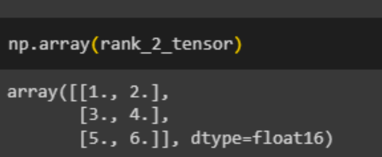
A tensor can be converted into a NumPy array using either np.array or the tensor.numpy method:

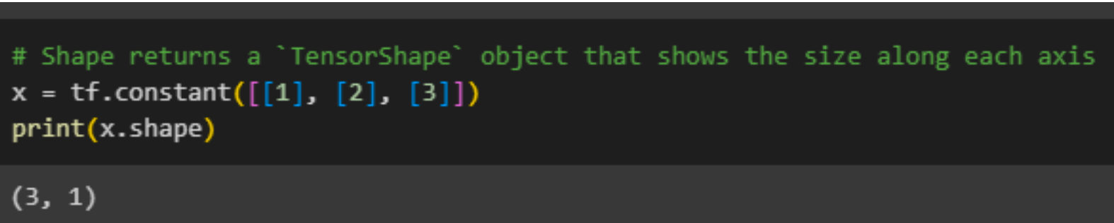
Some of the previous images contain the word shape, what is shape?Tensors have shapes: Shape: The count of elements along each axis of a tensor. Rank: The total number of axes in a tensor. Scalars are rank 0, vectors rank 1, and matrices rank 2. Axis or Dimension: A specific dimension within a tensor. Size: The overall quantity of items in the tensor, determined by multiplying the elements of the shape vector.

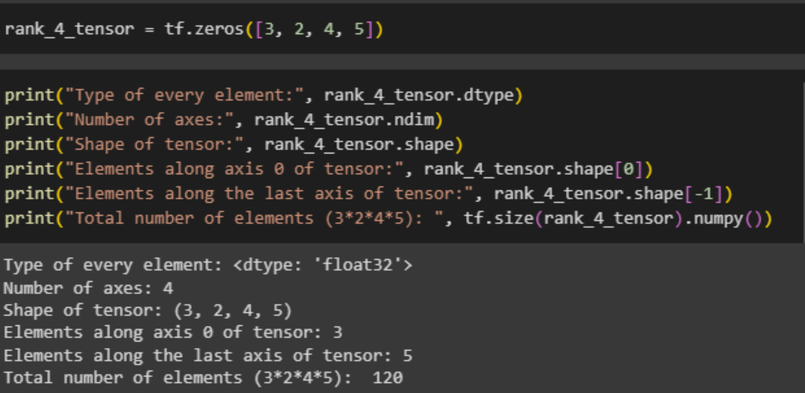
tf.zeros can be used to create Tensors that contain zeros with the provided shape.

More about shapes:

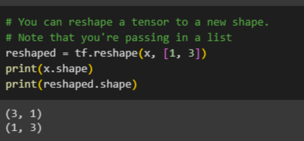
A tensor can be reshaped into a different shape. The tf.reshape function is efficient and cost-effective, as it doesn't require duplicating the original data.

Linear Regression: Linear Regression is a fundamental algorithm in data science. It is used to predict the association between two variables based on the presumption of a linear link between the independent and dependent variables. Its goal is to find the best-fit line that reduces the total squared differences between the predicted and actual values.

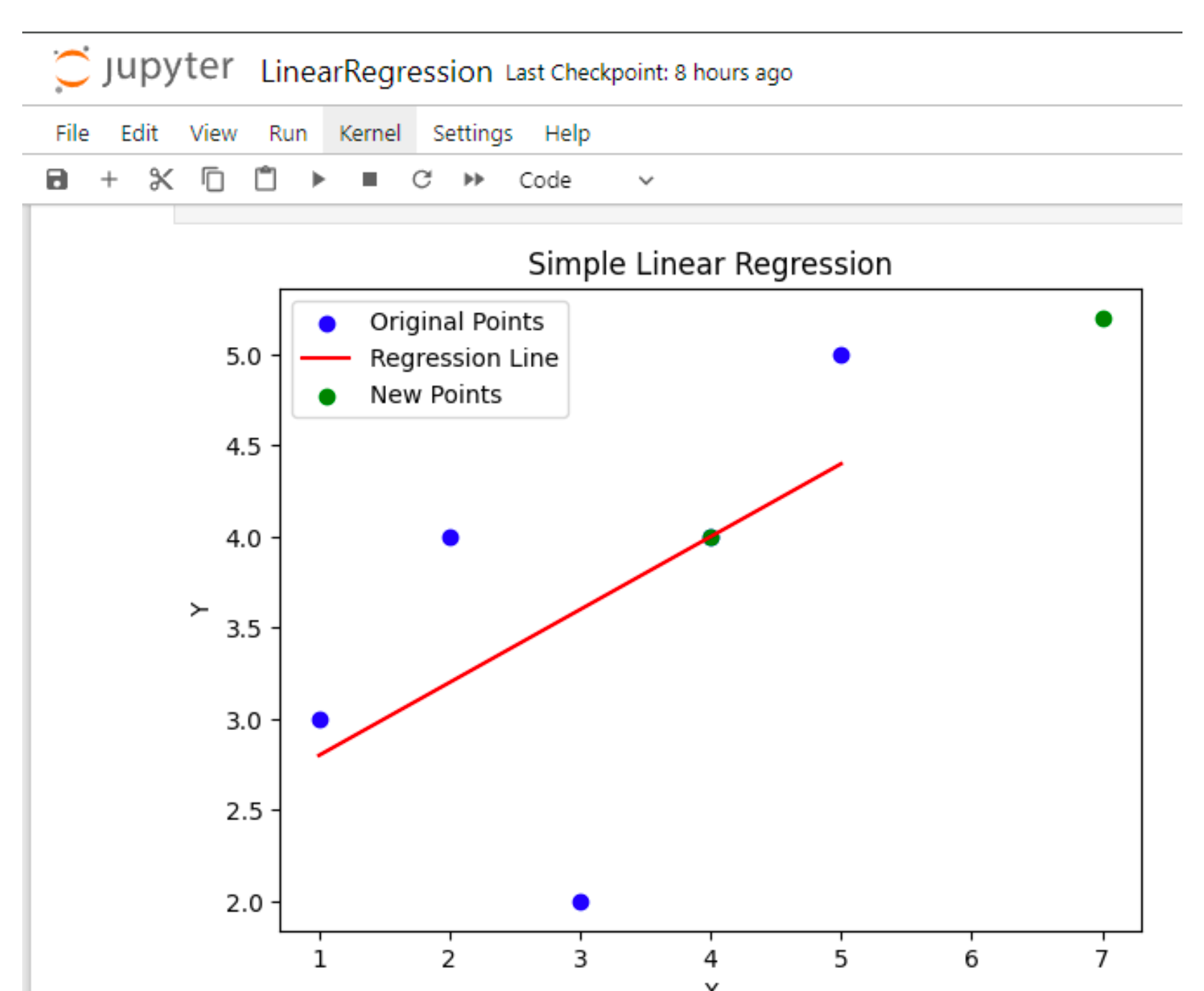
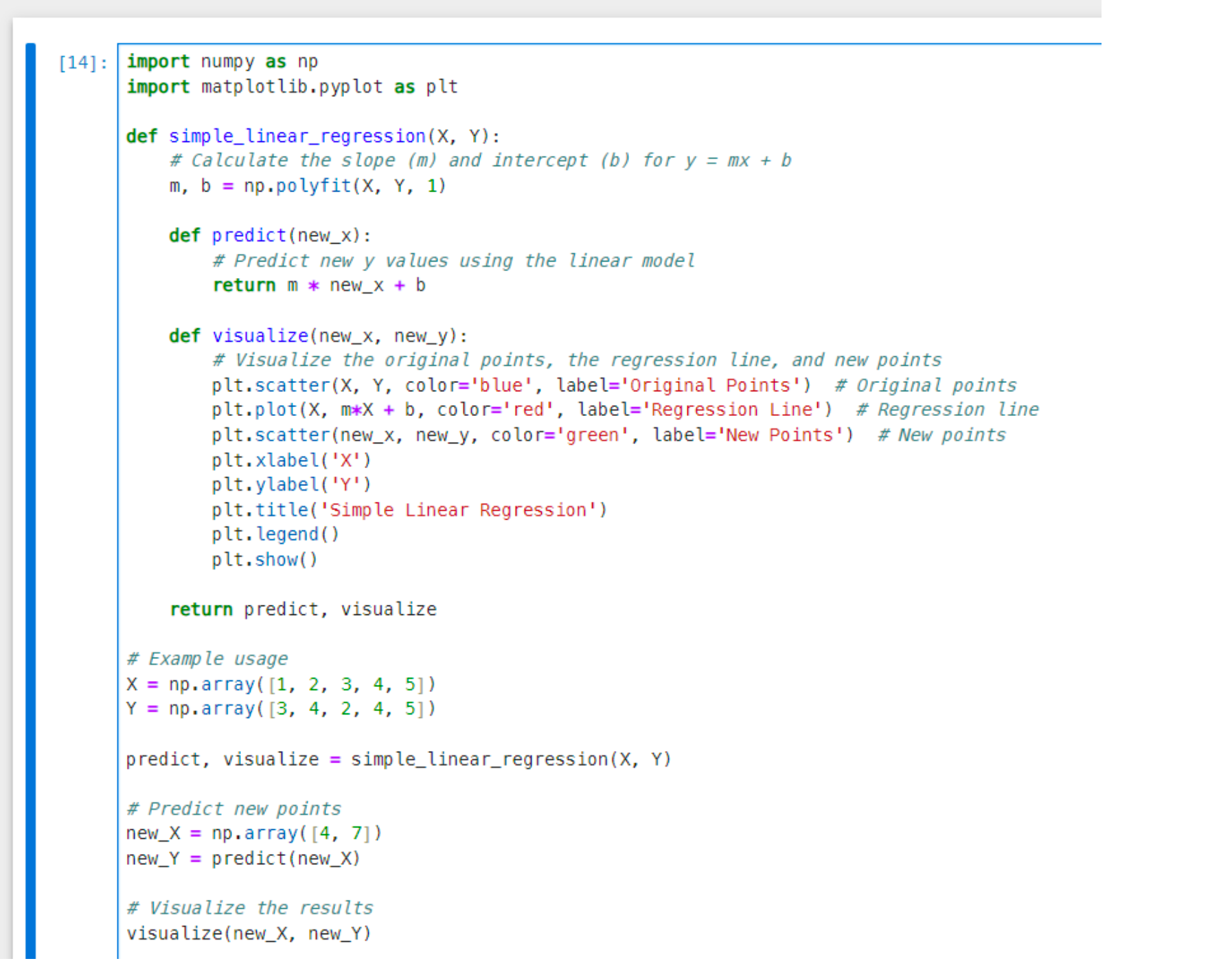
The blue dots are the training data that was provided to the function, based on the training data, this function creates a line that minimize the destination between the line and the dots. Then, the line will be used to predict new values. As you can see, the line was created based on the training data, and after we try to predict new values, it puts them on the line (green dots). Here is the code for this output:

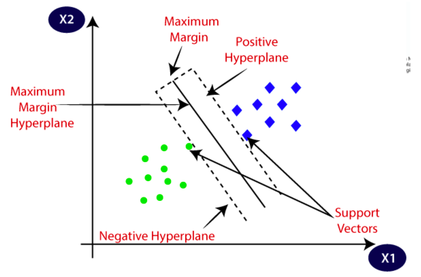
Support Vector Machines: Support vector machines (SVMs) is a famous supervised ML method that is being used for classification and outliers’ detection. One of the advantages of Support vector machines is that it works with low and high dimensional spaces. SVM focuses on identifying a hyperplane that optimally separates two classes. SVM is similar to logistic regression, however it is important to highlight that their approach differ fundamentally. Which hyperplane does it select? There can be millions of hyperplanes can classify the objects into 2 categories. So, how does SVM know which is the best?

SVM picks the best hyperplane by finding the maximum margin between the hyperplanes. This means that it selects the maximum distance between 2 objects (classes). SVM algorithms can be categorized into two types:

• Linear SVM: This is used when the dataset can be linearly separable, meaning that the data points can be classified into two categories with a single straight line.
• Non-Linear SVM: This is used when the dataset is not linearly separable, meaning the data points cannot be divided into two classes using a straight line in a two-dimensional view, we use Non-Linear SVM.

The main terms in SVM are:

• Support Vectors: These are the closest data points to the hyperplane in an SVM mode. The position of the hyperplane is mainly influenced by these points.
• Margin: This is the gap between the hyperplane and the nearest data points (the support vectors).

Bias: It can be referred to the errors in a machine learning algorithm. High bias means bad algorithm as it is more likely to give wrong predictions.

Variance: High variance means that the algorithm is not consistent with multiple datasets, in some datasets it has low bias, and in others it has high bias.

Cross validation: This helps to choose the best machine learning method for a specific purpose. It allows us to compare different machine learning methods and get a sense of how well they will work. When trying to choose the best ML method, we train 80% of the dataset and 20% to test the accuracy of the dataset. However, how to know which piece of data to train and which to test? Cross validation solves this problem by training and testing all the pieces in the dataset and return the best fit.

Kernel tricks: It transforms the dataset into a higher dimension where a hyperplane can effectively separate the classes.

Now, to understand SVM more, I will write simple Python code that uses SVM.

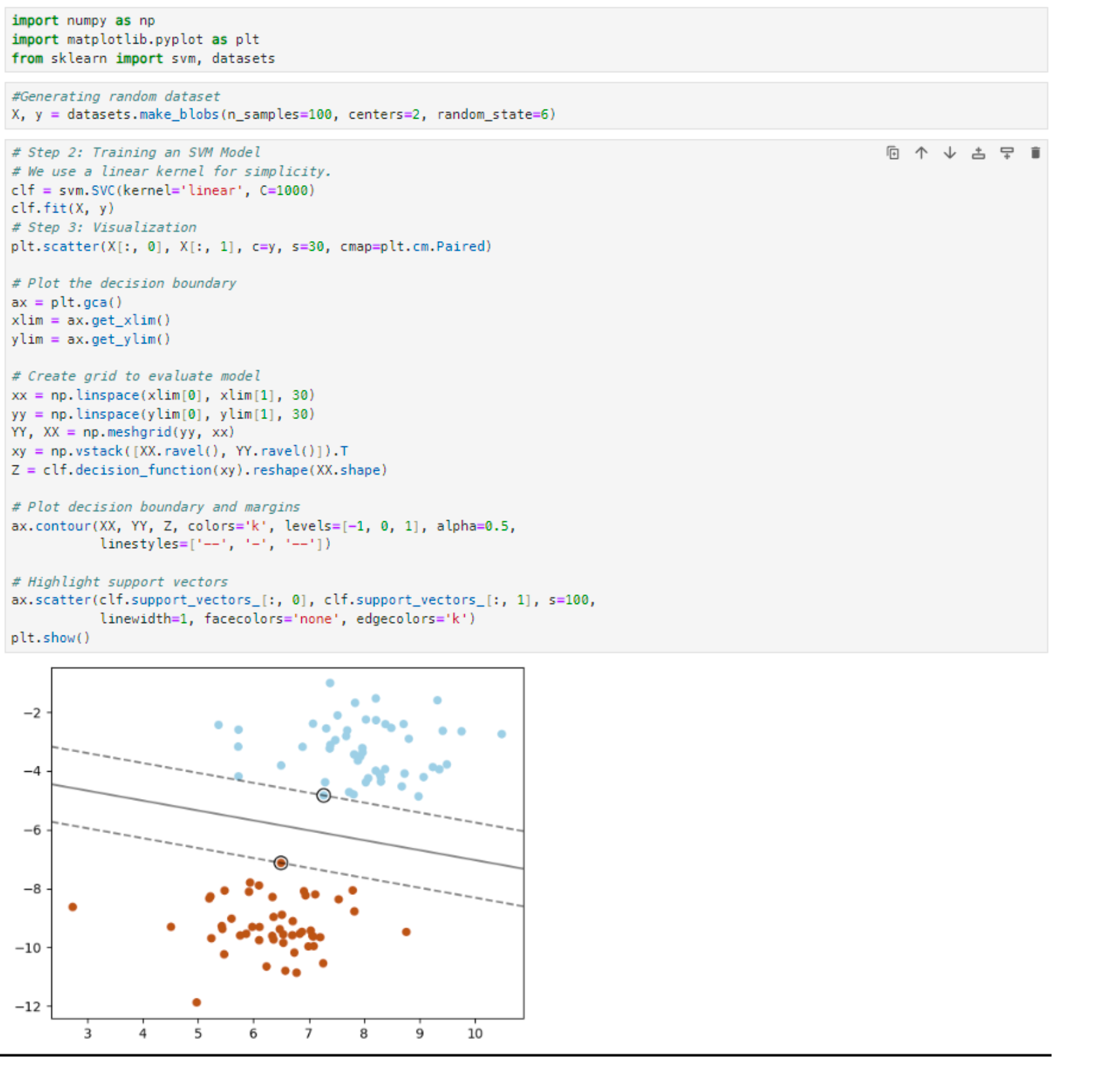
This is Jupyter notebook that implements a very basic SVM model. The plot shows that the model creates a hyperplane based on the distance between the closest data points.

Now, I want to make the model classifies (predicts) new data points. I added a new array that contains new data points that I want the model to classify:

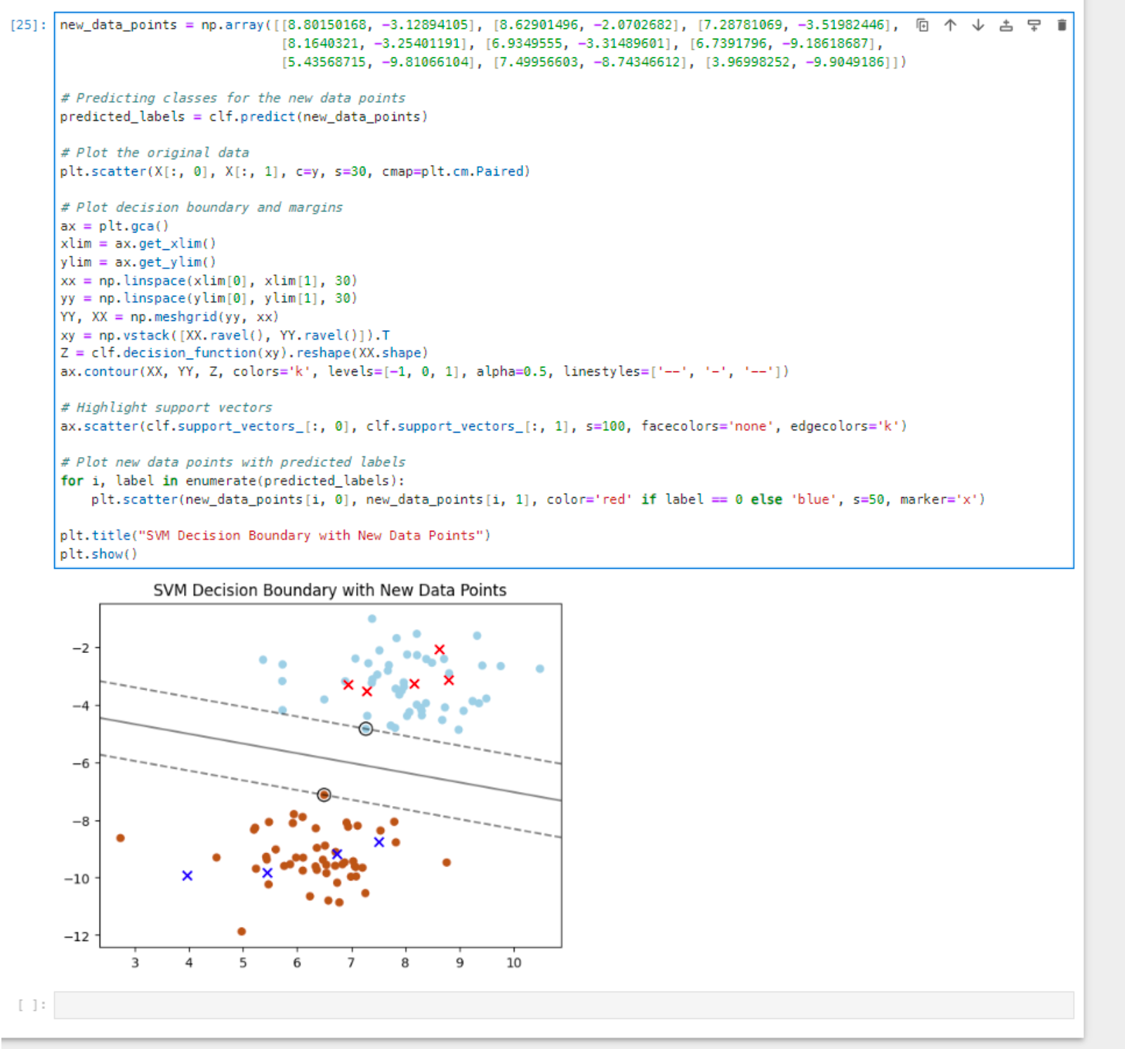
As seen above, the model predicts the location of the new data points and place them in their correct class.

Conclusion

Understanding the nature of entropy and information gain, as illustrated through the decision tree model, allows cyber security professionals to implement effective anomaly detection systems. With the right approach to training and the application of concepts like entropy in supervised learning, machine learning models can be trained to recognize and flag unusual patterns in network logs that could indicate a security threat. Furthermore, the integration of machine learning within big datasets would enhance the capability to automate the detection of anomalies in network traffic. By employing models such as decision trees, support vector machines, and others, organizations can effectively respond to potential cyber security incidents.

Question 2

How does Exploratory Data Analysis (EDA) contribute to understanding the NSL-KDD dataset, and what insights can it provide to inform the development of a more accurate intrusion detection model?

What is EDA?

Data scientists utilize exploratory data analysis (EDA) to examine datasets, highlighting their key features frequently using data visualization techniques. EDA helps determine the best methods for processing data sources to extract the necessary insights, making it easier for data scientists to find patterns, spot anomalies, test theories, or confirm presumptions. EDA's primary goal is to assist in examining data before drawing any conclusions. It can assist in locating glaring errors, better understanding data patterns, spotting outliers or unusual occurrences, and discovering intriguing correlations between the variables. Exploratory analysis is a tool that data scientists can use to make sure the results they generate are reliable and relevant to any intended business objectives. By ensuring that stakeholders are asking appropriate inquiries, EDA also benefits them. Standard deviations, categorical variables, and confidence intervals are among the topics that EDA can assist with. The features of EDA can be applied to more complex data analysis or modeling, such as machine learning, after it is finished, and conclusions have been drawn.

Exploratory data analysis tools

With EDA tools, you can perform a range of statistical procedures and methods, such as:

• methods for dimension reduction and clustering that help to visualize high-dimensional data with lots of different variables.
• presentation of individual attribute visualizations from the raw data set combined with summary statistics.
• Multivariate visualizations are useful for understanding and mapping the relationships between various data fields.
• K-means clustering is an unsupervised learning clustering technique in which data points are grouped into K groups, or the total number of clusters, according to how far they are from the centroid of each group. The data points that fall into the same category are those that are closest to a given centroid. Pattern recognition, picture compression, and market segmentation are three common applications of K-means clustering.
• Data and statistics are used by predictive models, like linear regression, to forecast outcomes.

Understanding the NSL-KDD Dataset

Dataset Overview

Tavallaee et al. (2009) state that the NSL-KDD dataset is a publicly accessible resource that was created from the previous KDD Cup99 dataset. An inaccurate assessment of Automated Intrusion Detection Systems (AIDS) resulted from a statistical analysis of the Cup99 dataset, which revealed important problems that significantly impact intrusion detection accuracy. The primary issue with the KDD dataset, as analyzed by Tavallaee et al. (2009), is the substantial number of duplicate packets present. Their analysis of both the training and testing sets revealed that approximately 78% and 75% of network packets, respectively, were duplicates.

Because there are a lot of duplicate instances in the training set, machine learning techniques may be biased toward typical cases and unable to learn from the irregular instances, which frequently pose more serious risks to computer systems. Tavallaee et al. removed duplicate records from the KDD Cup'99 dataset in 2009 in order to create the NSL-KDD dataset, which addresses the issues found in that dataset. There are 125,973 records in the NSL-KDD training dataset and 22,544 records in the test dataset. Because of its manageable size, the NSL-KDD dataset can be used for research purposes without the need for random sampling, which has resulted in consistent and comparable results across studies. The NSL-KDD dataset has 41 attributes and includes 22 training intrusion attacks. Of these, a full set of features for analysis in intrusion detection research are provided by the 19 attributes that describe the nature of connections within the same host and the 21 attributes that relate to the characteristics of the connection. (Saylor Academy, 2023)

Feature Composition

To address the "Feature Composition" of the NSL-KDD dataset for intrusion detection systems, we dive into the types of features included in the dataset, their data types, and their relevance to identifying potential security threats. Here is a closer look at the NSL- KDD dataset's feature composition:

Types of Features in NSL-KDD

The NSL-KDD datasets includes 42 features (columns) including a label feature that categorizes each connection as either normal or an attack. The types of attacks are also subdivided into four categories:

• DoS (Denial of Service)
• R2L (Remote to Local)
• U2R (User to Root)
• Probe

All the features in the dataset can be categorized into three main types:

• Basic Features: Basic Features encompass attributes extracted directly from packet headers, such as connection duration, protocol type, service requested, and flag status, representing core network connection qualities easily identifiable from network traffic
• Content Features: Content Features analyze packet payloads for anomalies, such as failed login attempts, crucial for detecting U2R and R2L attacks involving abnormal data transmissions.
• Traffic Features: These features track the connections where the same host is trying to connect to the same service. This can be helpful when trying to detect DoS attacks.

Data Types of Features

• Numerical Features: Most features in the dataset are numerical.
• Categorical Features: Some features are categorical, representing types of protocols (e.g., tcp, udp, icmp), services (e.g., http, ftp, telnet), and network connection status (e.g., SF, S1, REJ). These features often require preprocessing, to be used effectively in machine learning models.

Identifying Key Features

The dataset contains over 40 columns, making it important to choose only the key features that are relevant to determining if a particular connection is an attack or benign.

Using my knowledge of cybersecurity, I carefully looked over each column in the dataset and chose a few features that seemed relevant to my objective. The selected features and their descriptions are listed below:

• ‘duration’: The length of the connection.
• ‘protocol_type’: The type of the used protocol like tcp, udp, etc.
• ‘service’: The network service like http, telnet, ssh, etc.
• ‘flag’: The status of the connection like S0, S1, etc.
• ‘src_bytes’: The number of the data bytes from source to destination.
• ‘dst_bytes’: The number of data bytes from destination to source.
• ‘logged_in’: This is binary column where 1 means a successfully login and 0 otherwise.
• ‘is_host_login’: This is binary column where 1 means the login belonged to the "host" list and 0 otherwise.
• ‘is_guest_login’: 1 if the login is a "guest" login and 0 otherwise.
• ‘attack’: There is a column in the dataset that says whether that connection is normal or a type of an attack. There are many types of attack mentioned. Therefore, I will categorize all the type of attacks as only one value (attack) to make it a binary column (normal & attack).

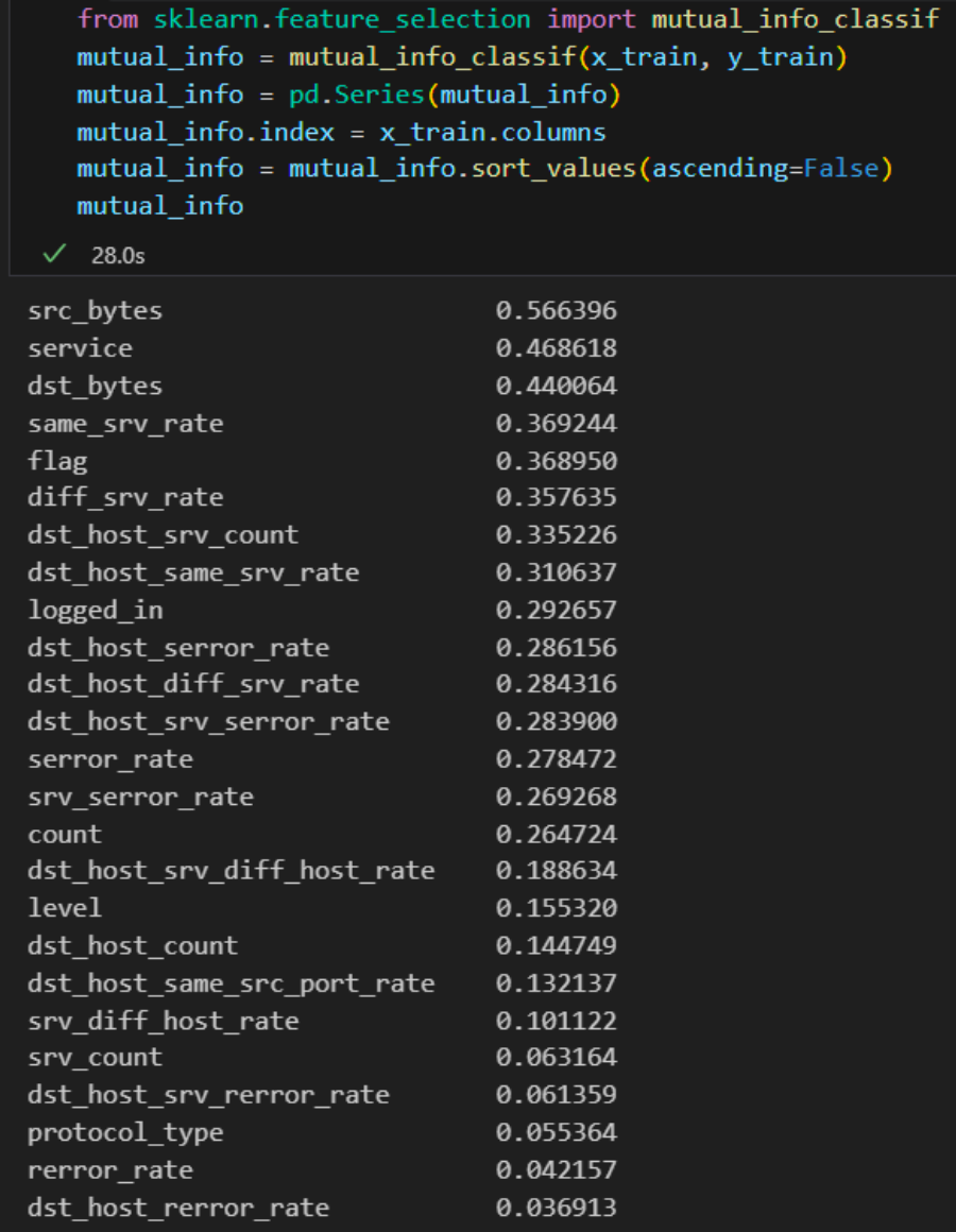
Identifying Key Features using Feature Selection

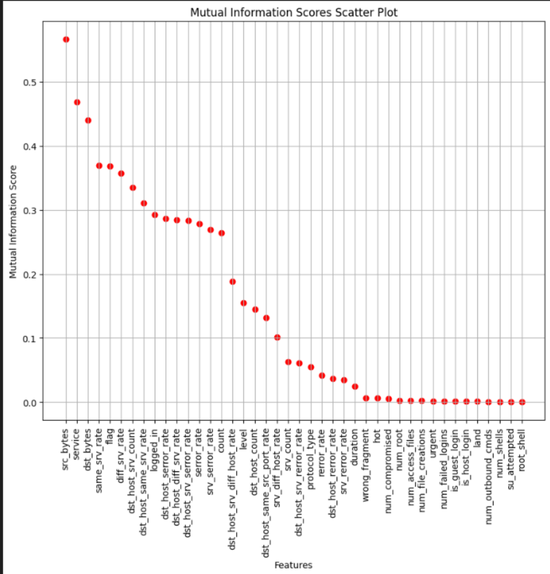
Hans mentioned that it is good to use my experience to pick the important features. However, he advised me to try and implement Feature Selection method to find the best possible features in my dataset. First, I will use mutual information classifier to evaluate feature importance. Then I will use SelectKBest to select the number of features that I want.

Here is a scatter plot that shows the most relevant features:

Then, I use SelectKBest to choose the features and assign them into new variable:

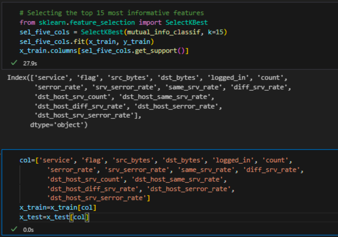
I faced an issue with the selected features; the machine learning models only handle numeric values, yet some of my features are in string format. In search of a solution, I discovered a technique known as One-hot encoding, which I will explore in the following chapter.

One-hot encoding

What is Categorical Data?

Categorical data refers to variables that carry label values instead of numerical ones. Normally, the values are in a fixed set.

• A “pet” variable might include options like “dog” and “cat”.
• A “color” variable could offer choices such as “red”, “green”, and “blue”.
• A “place” variable might list rankings like “first”, “second”, and “third”.

The Problem with Categorical Data

Some algorithms are meant to work with categorical data straight out of the box. Decision trees, for example, have the ability to learn directly from categorical data. But a lot of machine learning algorithms aren't designed to handle label data in its original form. They demand that the variables be presented in numerical form for both the input and the output.

How to Convert Categorical Data to Numerical Data?

Integer Encoding In the first phase of preparing categorical data for machine learning models, each unique category is assigned a specific integer. For example, the assignment could be set up so that "blue" goes with 3, "green" with 2, and "red" with 1. This is called integer encoding or label encoding, and it is easily reversed. This method might be more than suitable for some kinds of data.

Some machine learning algorithms can identify and make use of a naturally ordered relationship in the numerical values assigned by this method. This is especially true for ordinal variables, where the values' order has significance. An illustration of this would be the previously discussed "place" variable, for which label encoding accurately captures the first, second, and third categories' natural order, making it a useful technique for variables of this type.

One-Hot Encoding

For categorical variables where no such ordinal relationship exists, the integer encoding is not enough. Label encoding, which simply assigns integers to categorical variables without a foundational ordinal relationship, may not be the optimal approach for these variables. The model's performance may suffer or unexpected results, like predictions that fall illogically between categories, may result from relying too heavily on integer encoding, which could lead to incorrect inference of a natural order among categories. To address this issue, one-hot encoding is employed as an alternative strategy. This approach involves replacing the integer-encoded variable with new binary variables, each representing a unique category value. Essentially, for every unique category, a distinct binary variable is created: this variable is set to "1" for its corresponding category and "0" for all others.

Given the three categories ("red", "green", and "blue") in the "color" example, one-hot encoding would produce three binary variables. For example, if the color is "green," the encoding would be [0, 1, 0], where "green" is indicated by a "1" in the second position, and "red" and "blue" are represented by "0" in the first and last positions, respectively. This approach captures each category's existence or absence efficiently without suggesting a hierarchy. (Brownlee, 2020)

Conclusion

Based on the comprehensive analysis of Exploratory Data Analysis (EDA) and its critical role in data science, as well as the detailed exploration of the NSL-KDD dataset for intrusion detection systems, we can draw several conclusions. An essential first step in the data analysis process is exploratory data analysis. It gives data scientists the knowledge and resources they need to fully comprehend their dataset, find underlying patterns, spot anomalies, and test theories. EDA facilitates the effective communication of the story of the data through a variety of statistical methods and data visualization techniques, enabling well-informed decision-making and strategic planning. The importance of EDA is found in its capacity to direct the choice of suitable modeling and data processing methods, guaranteeing that the analysis is in line with the current business goals and inquiries. The investigation of one-hot encoding provides additional insight into the problems and solutions related to categorical data preprocessing for machine learning. Data scientists can fully utilize their datasets by converting categorical data into a format that machine learning algorithms can understand. This allows for more precise and insightful analysis. To sum up, the examination of EDA and its utilization with the NSL-KDD dataset highlights how interconnected preprocessing, feature selection, and data preparation are within the larger fields of cybersecurity and data science. It emphasizes the need for thorough data preparation and analysis as the first steps in obtaining trustworthy, useful insights, especially in domains where accuracy and precision are critical. This all-encompassing method not only makes it easier to comprehend the data at hand more deeply, but it also establishes the foundation for the creation of successful models and tactics, which in turn promotes advancements in cybersecurity and other fields.

Question 3

What are some effective machine learning models for intrusion detection in cybersecurity, and how do they compare in terms of accuracy, performance, and scalability when applied to the NSL-KDD dataset?

Machine learning primarily deals with two problem types: classification and prediction. Here is a compilation of commonly used algorithms used for creating classification regression models:

Classification Models:

• Logistic Regression
• Naïve Bayes
• Decision Trees
• Random Forest
• K-nearest neighbor (KNN)
• Support Vector Machine

Regression models

• Linear regression
• Ridge regression
• Decision trees
• Random forest
• K-nearest neighbor (KNN)
• Neural network regression

Theoretical Approach: Common Classification Models

Logistic Regression

Despite its name, logistic regression is primarily utilized for binary classification problems, where data falls into two categories. Logistic regression often serves as an initial method for setting a baseline before exploring more complex models. The word “regression” appears in its name because it estimates the likelihood of an outcome being either 0 or 1 through a linear combination of features. (Choosing the Best Machine Learning Classification Model and Avoiding Overfitting, 2023)

Naive Bayes

You may want to use the naive Bayes algorithm if your task and data are relatively simple. When training data is limited, this classifier is a better option than nearest neighbor and logistic regression algorithms due to its high bias and low variance. Naive Bayes works especially well when memory and CPU resources are restricted. Its ease of use keeps it from overfitting, enabling quick training. Additionally, it functions well when fresh data is added on a regular basis. However, as data complexity and variance increase, you might find more sophisticated classifiers to be more effective. Naive Bayes' straightforward analysis may not support complex hypotheses. (Choosing the Best Machine Learning Classification Model and Avoiding Overfitting, 2023)

K-Nearest Neighbor

Categorizing data points by their proximity to others in a training set can be an effective classification method. The k-nearest neighbor (KNN) algorithm operates on the principle of "guilty by association. Because KNN is regarded as an instance-based lazy learner, it does not go through a traditional training phase. Rather, you feed the model with the training set and let it run in the background until you need it. The KNN model determines the given number of nearest neighbors (k) in response to a new query; for instance, if k = 5, it evaluates the class of the five closest neighbors. The model uses a vote process among these neighbors to decide which label is best for classification. It determines the mean of the values of the closest neighbors for regression tasks. Although KNN requires less time to train than other models, it can take longer to query and require more storage space, especially when the dataset grows. All training data is retained by this model, as opposed to just algorithmic representation.

Decision Trees

To understand how a decision tree predicts an outcome, start at the root (beginning) node, and follow the path down to a leaf node, which provides the response. Classification trees generate nominal outputs like true or false, while regression trees yield numeric responses. Decision trees offer clear visibility of the decision-making path from root to leaf, making them particularly helpful when results need to be explained to stakeholders. They are also relatively quick to execute. However, a primary drawback of decision trees is their propensity to overfit data. Ensemble methods, such as bagging, can mitigate this issue.

Support Vector Machine

When there are clear differences between the two classes in your dataset, you may want to use a support vector machine (SVM). The ideal hyperplane is the one that maximizes the margin between these classes and divides the data points of one class from those of another. This is how support vector machines (SVMs) operate. SVMs deal with datasets that have more than two classes by dividing the issue into several binary classification tasks that are each overseen by a different SVM. SVMs offer significant benefits. They are highly accurate and generally resistant to overfitting. Linear SVMs, in particular, are straightforward to interpret. Once trained, SVMs are very quick, allowing for the disposal of training data if memory is limited, making them suitable for environments with restricted resources. They also excel in complex, nonlinear classification tasks through the use of a technique known as the "kernel trick.

However, SVMs require considerable upfront training and tuning, necessitating a significant time investment before they can be deployed. Additionally, their performance can decrease when handling more than two classes, affecting their speed.

Neural Networks

An artificial neural network (ANN) is capable of learning and can be trained to solve problems, recognize patterns, classify data, and predict future events. ANNs are frequently employed for complex challenges like character recognition, stock market predictions, and image compression. The functionality of a neural network hinges on the architecture of its nodes and the strength of the connections between them, known as weights. These weights adjust automatically during training, adhering to specific learning rules until the network proficiently executes the intended task. ANNs excel in handling nonlinear data with numerous input features, making them ideal for tackling sophisticated problems that simpler algorithms struggle with. However, they come with some downsides: ANNs are resource-intensive, their decision-making processes are often opaque (making it hard to deduce how a solution was reached) and fine-tuning them can be impractical—you generally have to alter the training inputs and retrain the network entirely.

Practical Application: Common Classification Models

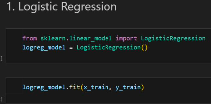
Logistic Regression

Importing and building the model.

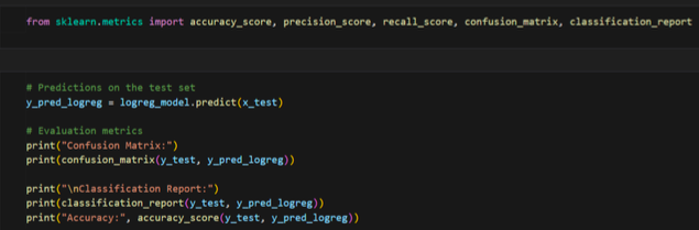
Evaluating the model

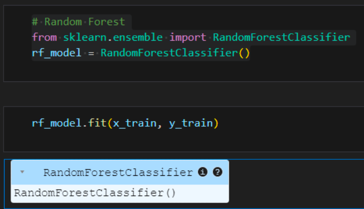
Random Forest Classifier

Importing and building the model

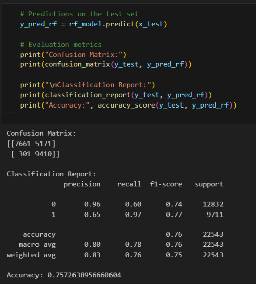
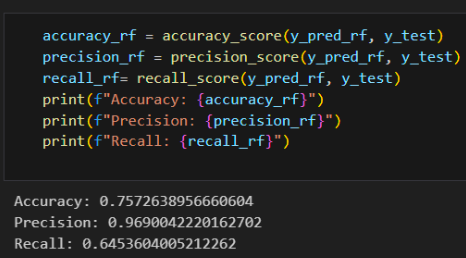
Evaluating the model

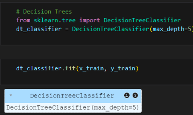
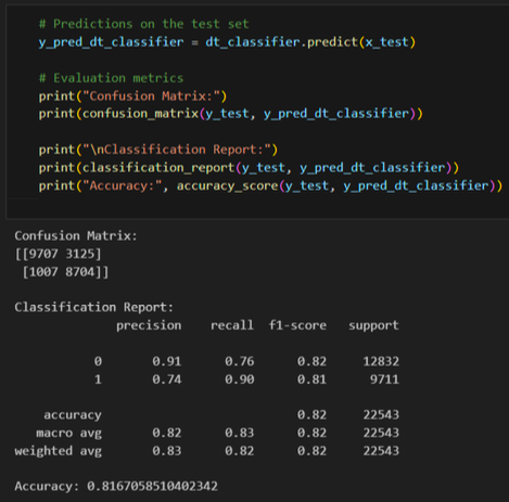
Decision Trees Classifier

Importing and building the model

Evaluating the model

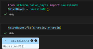
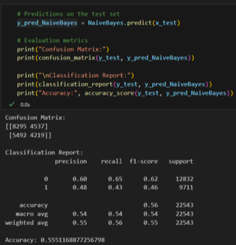
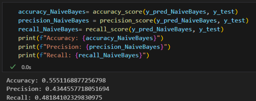
Naïve Bayes

Importing and building the model

Evaluating the model

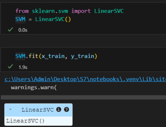
Support Vector Machines Linear

Importing and building the model

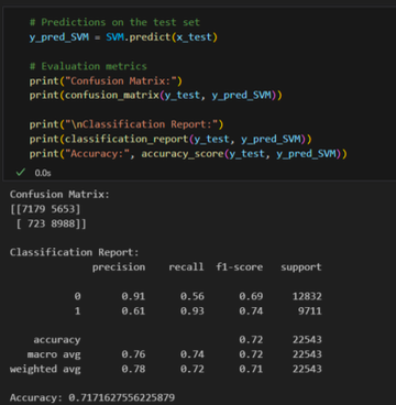
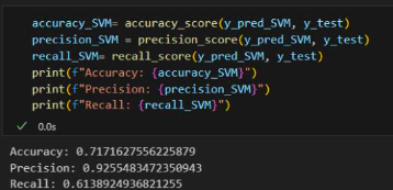
Evaluating the model

Models Evaluation

In cybersecurity, accurately identifying attacks is crucial. Misclassifying an attack as normal can cause severe damage, while misclassifying normal activity as an attack is less harmful. I've built five machine learning models to classify attacks in the NSL-KDD dataset, focusing on minimizing false negatives to enhance security.

For each ML model, I will provide the accuracy, precision, and recall. Additionally, I will include a heatmap showing True/False Positives/Negatives. Note: I aim to minimize false positives, as missing attacks in security is highly undesirable.

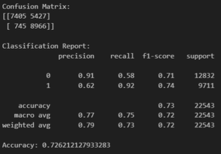
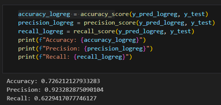
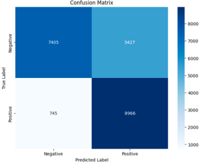
Logistic Regression

• Accuracy: 72%
• Precision: 92%
• Recall: 62%
• False Positive: 754

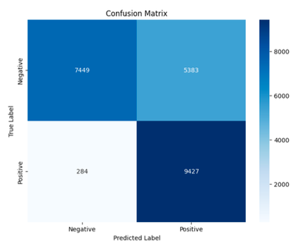
Random Forest Classifier

• Accuracy: 75%
• Precision: 97%
• Recall: 63%
• False Positive: 284

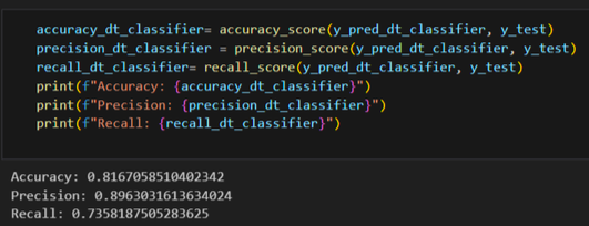
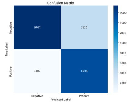
Decision Trees Classifier

• Accuracy: 81%
• Precision: 89%
• Recall: 73%
• False Positive: 1007

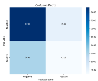
Naïve Bayes

• Accuracy: 55%
• Precision: 43%
• Recall: 48%
• False Positive: 5492

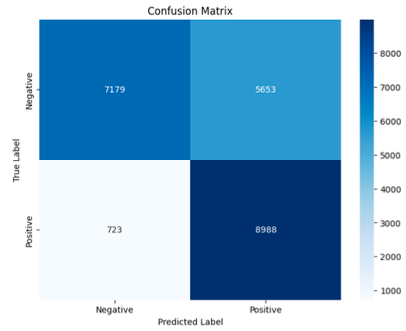
Support Vector Machine Linear

• Accuracy: 71%
• Precision: 92%
• Recall: 61%
• False Positive: 723

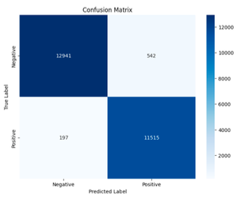
Neural Network

• Accuracy: 97.07%
• Precision: 97.11%
• Recall: 97.07%
• False Positive: 197

Conclusion

In evaluating the performance of six machine learning models for classifying attacks in the NSL-KDD dataset, a key focus has been on minimizing false positives to ensure high security. Each model was assessed for accuracy, precision, and recall, alongside a detailed analysis of false positives and negatives.

Among the models tested, the Neural Network demonstrated superior performance with an accuracy of 96.01%, a precision of 96.27%, and a recall of 96.01%, while maintaining the lowest number of false positives at 47. This indicates its strong capability in accurately identifying attacks and minimizing false alarms, which is critical in a cybersecurity context.

The Random Forest Classifier also showed promising results with high precision (97%) and relatively low false positives (284), though it lagged in recall (63%). Other models, such as Logistic Regression and Support Vector Machine Linear, offered good precision but were less effective in recall and had higher false positives compared to the Neural Network.

Overall, the Neural Network model stands out as the most effective for this task, striking the best balance between accuracy, precision, and recall, while minimizing the risk of false positives. This makes it a highly suitable choice for enhancing security by reliably detecting attacks without overwhelming with false alerts.